Statistical model for cancer diagnoses

The 'expected' incidence (number of new cancer diagnoses) of a postal code area

The data described under ‘Cancer and population data’ were used to estimate standardized incidence ratios (SIR) for each area in the Netherlands using statistical models.

The SIR is the ratio of the observed number of cancer diagnoses in an area to the expected number of diagnoses in that area. The expected number of cancer diagnoses is the number of diagnoses that is expected in an area if the risk of cancer would be uniform throughout the Netherlands. This calculation takes into account the number of people living in an area and their age. In areas with many residents, there is generally a higher incidence of cancer than in areas with few residents. Similarly, as an area with a relatively higher proportion of older individuals will contain more cancer cases than an area with a younger population. By accounting for these effects of age and population size differences, they should no longer be visible in the final atlas.

To estimate the SIR, we first calculate the average number of cancer diagnoses in the Netherlands per age category and per person (or per 100,000 persons). This is known as the age-specific incidence rate. If the risk is the same throughout the Netherlands, we expect that the age-specific incidence rates in every area are approximately the same. If we know how many people of each age live in an area, we can estimate how many cancer diagnoses we would expect in that area if the age-specific incidence rates in that area are the same as those in the Netherlands. To this end, we multiply the Dutch age-specific incidence rate for each age category by the number of people living in the area of interest. By then summing the expected number of cancer diagnoses per age category, we get the total absolute number of expected cancer diagnoses in that area. The formula for this is as follows:

E_i is the expected number of cancer diagnoses in area i. 'a' represents the age category: age category 1 includes ages 0-5, and age category 18 includes ages 85 and older. This calculation is a form of indirect standardisation, ensuring that differences between areas are not attributable to an older or younger population in those areas or differences in population size between areas. Subsequently, the observed incidence in this area is compared with the expected incidence. This requires a statistical model.

(Un)certainty around the incidence - Areas with few residents

By comparing the observed incidence in each area with the expected incidence, we determine whether this area has a higher or lower incidence than expected based on the Dutch average, the population size and age distribution of the specific area.

However, not every area contains the same number of residents and the same number of cancer diagnoses. Areas with few residents and/or few cancer diagnoses can especially distort the picture and blur the underlying geographical patterns. The cancer incidence in areas with few residents and/or few cancer diagnoses is more susceptible to random fluctuations than in areas with more residents and/or a higher incidence. A difference of 1 cancer diagnosis has a much more significant impact in an area with a low incidence than in an area with a high incidence.

In a hypothetical and simplified example: if 3 cancer diagnoses are observed in a small area where 2 diagnoses are expected (SIR = 3/2 = 1.5), the incidence appears 50% higher than expected. But in a larger area where 30 cancer diagnoses are observed and 29 are expected (SIR = 30/29 = 1.03), the incidence is only 3% higher than expected. Small areas can thus cause extreme outliers in this way, while differences sometimes simply arise from randomness. Smoothing leads to more stable estimates of the SIR. Additionally, the uncertainty around an estimated SIR is often greater in areas with few residents and/or few cancer cases. This is because there is less data available for estimating the SIR. Smoothing not only ensures a more stable SIR but also often reduces the uncertainty around the estimated SIR. In general, smoothing ensures that extreme outliers become less extreme and their uncertainty becomes smaller. This results in a more stable and realistic depiction of the geographical pattern of cancer incidence. See Figure 7a for an example of how smoothing works.

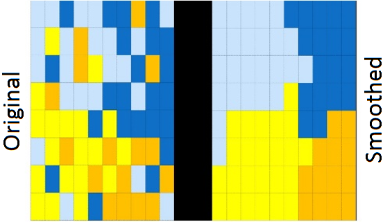
Figure 7a. Left: observed incidence. Right: incidence with smoothing.

For the Dutch Cancer Atlas, we follow the methodology that was used for the Australian Cancer Atlas. We use a Bayesian model with a Conditional Autoregressive (CAR) Distribution.

Statistical model

We assume that the observed incidence (number of new cancer diagnoses) Yi in area i follows a Poisson distribution (a particular probability distribution):

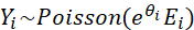
where E_i  is the number of expected cancer diagnoses and θ_i  is the natural logarithm of the standardized incidence ratio (SIR) in area i. When exponentiated, the value θ_i indicates the extent to which the incidence in an area deviates from the average: an SIR of 1 indicates that the incidence in an area is equal to what would be expected based on the Dutch average (1 * E_i = E_i). An SIR below 1 indicates that an area has a lower incidence than expected based on the Dutch average and an SIR above 1 indicates a higher incidence than expected.

These SIR values are displayed in the Dutch Cancer Atlas, along with their uncertainty. The logarithm of the SIR is then parameterized as:

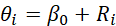
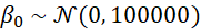
The parameter β₀ represents the average SIR and R_i ​​​​ is known as a spatial ‘random effect’, representing the extent to which area i deviates from this average. The specification of these spatial random effects determines how smoothing is performed. In Bayesian models, priors are specified, which are also known as a priori distributions. These priors reflect our level of knowledge before processing the data. This knowledge is then updated as the model processes the data, leading to a posterior distribution. The a priori distribution for β₀ is normally distributed with a mean of 0 (because e⁰ = 1: on average areas will match the Dutch average) and a very wide variance. The latter implies that we want to assume little about the data beforehand, allowing the data to have a significant impact on our final estimate.

The spatial random effects R_i ​​​​ follow a distribution as proposed by Leroux et al. 2000; these values are a weighted average that also take into account the values of random effects from neighbouring areas. This is how the aforementioned ‘smoothing’ takes place;

 and also ρ have a so-called a priori distribution, which can then be more precisely estimated using the observed data. The a priori distribution for follows an inverse gamma distribution with shape parameter 1 and scale parameter 0.01:

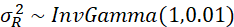
Here too a scale parameter of 0.01 means that we assume very little beforehand about the values and thus assign a lot of weight to the observed data. Finally, the a priori distribution for ρ;

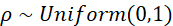
A ρ of 0 would mean there is no spatial correlation (each area is independent of its neighbouring areas) and a ρ of 1 would mean that there is a fully dependent relationship. By assuming a uniform distribution from 0 to 1, every possible value between 0 and 1 is possible; here the data also have a strong influence on the estimation.

Reference

Leroux BG, Lei X, Breslow N. Estimation of disease rates in small areas: a new mixed model for spatial dependence. 2000. 135-178. In Halloran ME, Berry D (Eds). Statistical models in epidemiology, the environment and clinical trials. New York: Springer.